NX7U
Scott Townley
Bridgewater, NJ
Feed Blockage in a Prime-Focus Parabolic Reflector Antenna
Determination by Integration of the Aperture Distribution
Unblocked Case
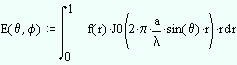
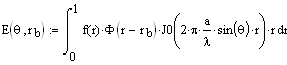
The secondary (feed+reflector) radiation pattern of a circularly-symmetric parabolic reflector antenna fed with an axially symmetric antenna located at the reflector focus is given by the integration:
Equation 1
where f(r) is the illumination function, J0 is the Bessel function of order zero, and the normalized variable r is the projected aperture of the reflector (the focus would lie on r = 0, the center of the aperture, and the edges of the reflector lie at r = 1). a is the size of the aperture, which is normalized to wavelength.
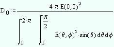
Equation 1 then gives the secondary pattern, but to find the directivity (in order to assess the effects of blockage), we need to integrate again:
Equation 2
where E(0,0) is meant to be the maximum field intensity over E(theta, phi). Note the theta integration is only in the upper hemisphere; the pattern representation in Equation 1 is only valid in front of the reflector (so it cannot be used to calculate backlobes or any sort of back radiation).
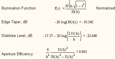
So all we're missing is a functional description of the feed illumination. Hansen [1] came up with a clever one-paremeter analytical function that is a close match to actual feed patterns. The function has the advantage that with a single parameter "h", the distribution, resultant sidelobe level, edge taper, and aperture/illumination efficiency can all be calculated in closed form by simple arithmetic...mostly.
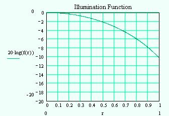
Here is an example, where h=2.5
I0(x) and I1(x) are the modified Bessel functions of order 0 and 1. Microsoft Excel will calculate these! The functions are Besseli(x,0) and Besseli(x,1). Make sure you have the "Analysis ToolPak" loaded.
Here is a graph of f(r) for the example distribution above. The edge illumination of -10.3 dB would be a relatively high gain design target. Note that as h is increased, the edge taper increases (more taper), the sidelobe level goes down, but the aperture efficiency goes down as well. You trade gain for sidelobe level with h (that's generally true with any description of the illumination function, not just Hansen's).
It's interesting that there is a closed-form expression for aperture efficiency. Note however that there isn't an equivalent expression for spilloverin fact, you can't even calculate spillover "brute-force" because the illumination function isn't defined for r>1.
Blocked Case
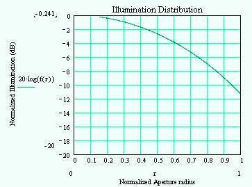
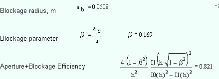
Now consider the presence of a blockage. The blockage essentially "darkens" the illumination distribution between r = 0 and B = ab/r = the radius of the blockage, normalized by the radius of the reflector (e.g., a 100 cm reflector with a 10cm blockage would be described by B = 0.1, or 10% blockage).
The line in the illumination distribution should drop down to -infinity dB at r = 0.15 in the graph (but I can't quite get it to work out...). The resultant aperture illumination is "donut" shaped as a result. Note that the peak of the illumination function is -0.24dB rather than 0dB.
Amazingly enough, the additional loss in efficiency due to the blockage can be calculated in closed form (below). Of course since we have the aperture efficiency by itself from the unblocked case, we can calculate the loss of efficiency due to blockage alone by BlockageLoss=10*log(0.821/0.903)=-0.41dB.
Note the dimensions given would be for a typical 60cm center-fed dish (feed blockage diameter = 4" or 10 cm). But it is equally valid for a 120 cm dish blocked by 20 cm, or for a 2.5 m TVRO dish using a tri-band patch feed (diameter=42 cm)! Only the ratio of blockage diameter/dish diameter matters.
Sidelobe Effects
Blockage also impacts the secondary pattern of the antenna, by raising the sidelobe level. Eqn. 1 would be modified:
The added function F(r-rb) in Mathcad is a "step-function". When the argument (r-rb) is less than zero, F is zero. When the argument is greater than or equal to zero, F is 1. Basically, the step-function "blanks out" the field of the illumination function f(r) between 0 and rb, the (normalized) radius of the blockage.
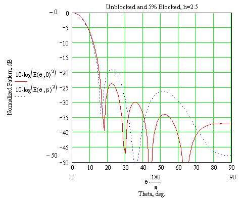
This chart shows the radiation pattern for both the unblocked (solid red) and blocked (dashed blue) case. Note the higher sidelobes at 22 degrees (+4.5dB) and at 50 degrees (+8dB).
As the edge taper is decreased (more taper/higher "h") the effect on sidelobe levels becomes more severe. That's because with all else equal, more total energy is blocked, because more energy is concentrated in the center of the feed pattern...which is blocked.
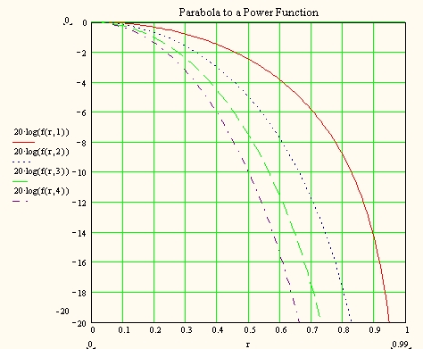
The "parabola-to-a-power" illumination function is f(r,p)=(1-r2)p. Note that the edge taper for this function is always -¥ dB. This function was useful for mathematical tractibility (it's easily integrated into Eqn. 1) before Hansen published his one-parameter method.
|
p |
aperture efficiency |
sidelobe level (chart below) |
|
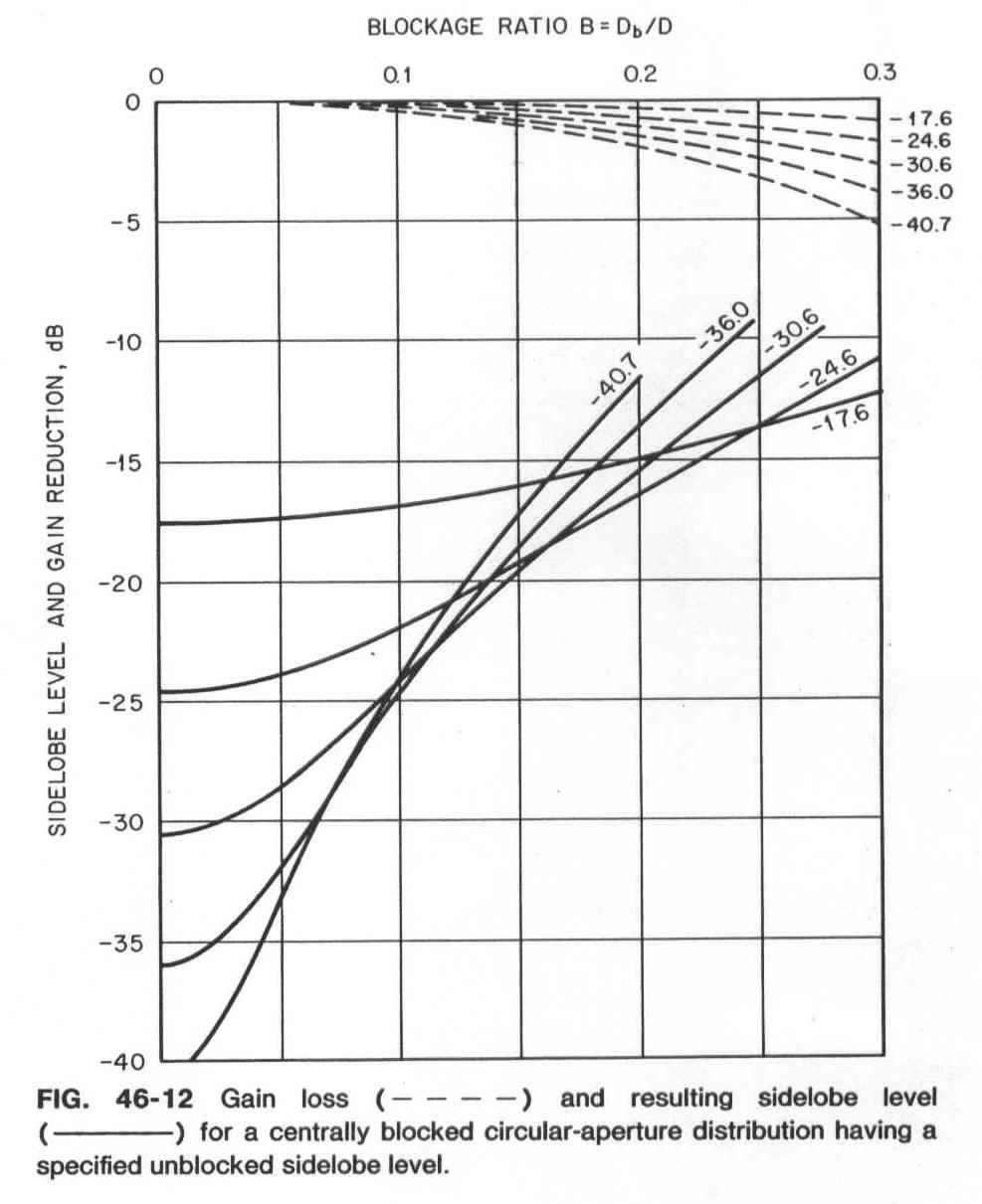
0 |
1.0 |
-17.6 dB (uniform dist.) |
|
1 |
0.75 |
-24.6 dB |
|
2 |
0.56 |
-30.6 dB |
|
3 |
0.40 |
-36.0 dB |
|
4 |
0.35 |
-40.7 dB |
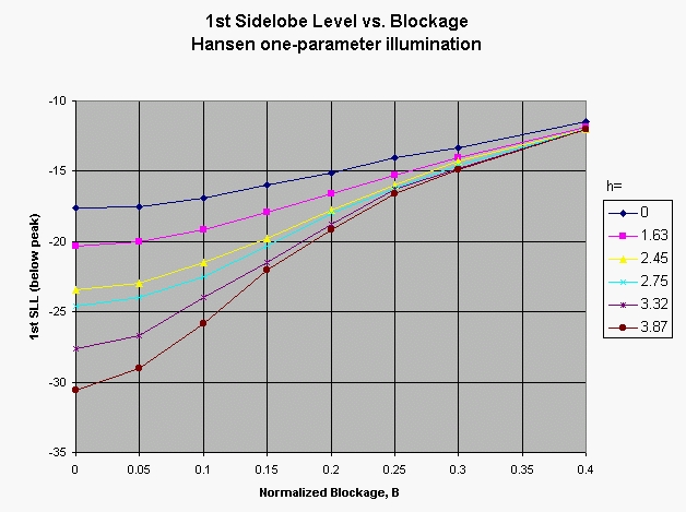
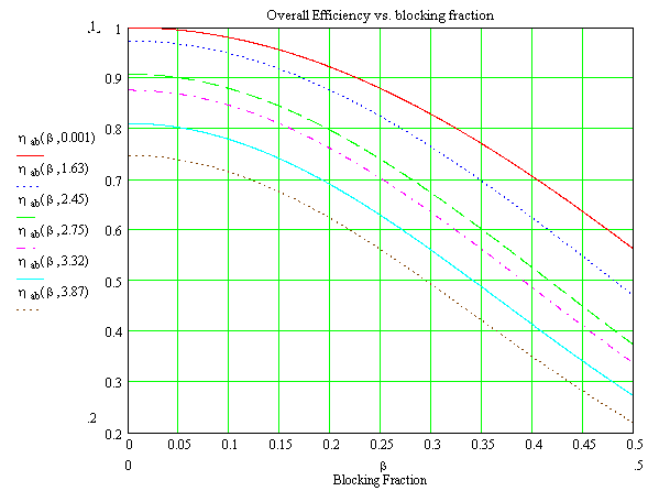
The above chart summarizes the total efficiencies (taper plus aperture blockage) obtained versus blockage for various tapers, or parameters "h". The values of "h" are chosen for specific edge illumination tapers summarized in the table to the right:
|
h |
edge taper |
nominal 1st sidelobe |
|
0 |
0 dB (uniform) |
-17.6 dB |
|
1.63 |
-5 dB |
-20.3 dB |
|
2.45 |
-10 dB |
-23.4 dB |
|
2.75 |
-12 dB |
-24.8 dB |
|
3.32 |
-16 dB |
-27.6 dB |
|
3.87 |
-20 dB |
-30.6 dB |
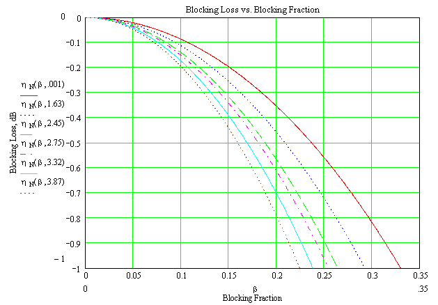
Similar to above, but now the scale is expanded, and the curves are recalculated for blocking loss only. Again, note that "lower-noise" feeds (more tapered; higher value of h) suffer more from blockage.
Conclusion
Blockage impacts both efficiency (gain) and sidelobe levels (antenna noise temperature). Both work against the link budget--with increasing blockage, gain goes down and antenna noise temperature goes up, so G/T decreases even more rapidly. The absolute size of the reflector doesn't matter, 25% blockage on a 20ft dish is just as bad as it is on a 2ft dish. Finally, for low-noise designs (e.g., EME), blockage must be kept to a very small value.
References
Another Viewpoint
Another analytical aperture illumination is the "parabola to a power". This illumination function is shown in the following chart. The analytical results for the secondary pattern of the "parabola to a power" is discussed in Johnson and Jasik (ed.), Antenna Engineering Handbook, 2nd. Edition, p. 46-23 and Fig. 46-12 below..
Hansen, R. C., "A One-Parameter Circular Aperture Distribution with Narrow Beam-Width and Low Sidelobes", IEEE Trans. Ant. Prop., July 1976, pp. 477-480.
Love, A. W., "Central Blocking in Symmetrical Cassegrain Reflectors", IEEE Ant. Prop. Magazine (Antenna Designer's Notebook), Feb. 1992, pp. 47-49.
How I Did It
All the equations, graphs and calculations were done using Mathworks' MathCad 11. One of my favorite toys.
A summary of the impact on sidelobe level due to blockage, using the same set of Hansen "h-" parameters as the loss calculations above. The design sidelobe level for the h=3.87 curve is -30.6dB, but a blockage ratio of 0.25 sets you back to the uniform illumination (h=0) case. You get all of the noise temperature of uniform illumination without the aperture efficiency!
Low sidelobe levels mean low antenna noise temperature, so a true "low-noise" design requires that blocking be kept quite low (B<0.05).
Summary Charts
This chart is very similar to my chart above for Hansen's distribution. The results here are a bit more pessimistic, but that's because the parabola-to-a-power distribution is more tapered than Hansen's (and we have seen that more taper results in more impacts due to blockage).
Note that once the blockage ratio B=0.15 or more, any design attempt at "low-noise" or low sidelobe levels is essentially wasted. All tapers give between -15dB and -20dB sidelobes.


")
")